Deep RL from Scratch

This project was associated with Northwestern University ME 469: Machine Learning and Artificial Intelligence for Robotics.

Introduction

Objective

The goal of this project was to learn pathfinding with RL. While A* is a widely used path planning algorithm in robotics, RL and other learning-based approaches can be model-free, more adaptive, and allow more optimization design choices.

Neural Network Overview

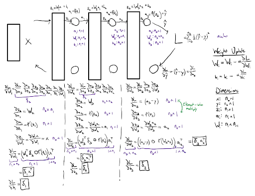
Deep RL algorithms use neural networks to approximate the RL value function or policy, so a custom neural network infrastructure was created for this purpose. The infrastructure is designed in the image of PyTorch’s autograd system, efficiently carrying out the backpropagation algorithm by recording relevant tensors during a network’s forward pass.

A fully connected neural network (FCNN) consists of several layers, with each layer possessing a matrix of weights and an activation function for the purpose of learning nonlinear relationships. In a network’s forward pass, inputs are transformed by a series of matrix multiplications and passed through the nonlinear activation functions to produce an output. This output is evaluated based on a target value using a loss function. The derivative of this loss function with respect to each layer’s weights is used to update the weights with the gradient descent algorithm in the backward pass. By iterating on this process, a network is able to learn complex behaviors from data. The math for the neural network implementation can be found in the figure below.

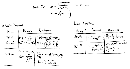
Neural networks require nonlinear activation functions to learn complex behaviors, and loss functions to evaluate their performance. This project includes implementations of the sigmoid, rectified linear unit (ReLU), and softmax activation functions. It also includes binary cross-entropy (BCE) and mean-squared error (MSE) loss functions. Weight initialization is another design decision in neural networks, with Xavier weight initialization being one of the most commonly used methods to improve training stability. The activation and loss function math can be found in the figure below.

RL Algorithm Overview

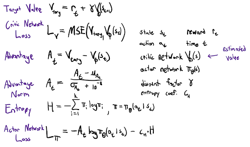
A2C is a deep RL algorithm that combines policy-based and value-based approaches. In this implementation, an actor network outputs a probability distribution over actions, while a critic network estimates the value function for each state. Practically, the final layer of the actor network uses a softmax activation function that forces it to output probabilities summing to one. The actor is trained using a loss proportional to the negative log-probability of the chosen action multiplied by the advantage, defined as the difference between observed returns and the critic’s estimate. An entropy term is added to the actor loss to act as a regularizer and an exploration incentive. The critic is trained to minimize the MSE between predicted and target state values. The math for this formulation can be found in Figure 6. Training can be performed on individual transitions or in batches of rollouts collected from the environment, and the advantage is normalized to reduce variance. Exploration is encouraged via a stochastic policy with an epsilon-greedy exploration probability, as well as the entropy term. Performance metrics, including average reward, advantage, and actor/critic losses, are logged and optionally visualized during training. The A2C math is in the figure below.

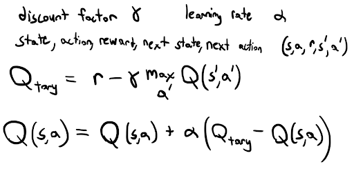
Also included is an implementation of tabular QL for a discretized 2D gridworld. States are mapped to discrete grid indices, and a Q-table stores the expected return for each state-action pair. The agent selects actions using an epsilon-greedy policy and updates the Q-values according to the standard QL update in Figure 7. Training occurs over multiple episodes, with each episode limited by a maximum number of steps. Episode statistics are logged and optionally printed. After training, the learned policy can be tested greedily to evaluate performance metrics such as average reward, average episode length, and success rate. The QL math is in the figure below.

Results

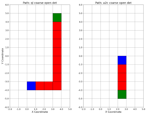
The ultimate goal for the two RL algorithms was learning task completion, with subgoals being lower training time, less expended energy, and a high success rate. The QL algorithm was successful at all of these goals; it achieved a 100 percent success rate on most random-start, fixed-goal permutations, and had the lowest training times. Perfect success rates were achieved in testing after longer training periods. It also exhibited significantly lower episode lengths when compared to the baseline performance in Table 1. A2C was also somewhat successful at these goals. It had a 100 percent success rate in the coarse grid resolution with and without obstacles, but the low average episode step count for both successful permutations suggests that the start and goal positions were relatively close. The figure below displays trial runs using both QL and A2C.

Grid resolution unsurprisingly also had an effect on training time and average episode length. The total training time and average episode length are greater in almost all cases on the fine grid resolution than they are on the coarse resolution. Increasing the grid resolution increases the size of the state space, so this data demonstrates that training time scales with state space size. A variety of FCNN sizes and architectures were also tested, with larger critic network sizes providing better performance but longer training times. Because actor loss calculations depend directly on critic value estimations, performance was generally better when the critic learning rate was faster or equal to that of the actor.

Because of its sample efficiency, QL was capable of quickly learning navigation from a randomized start location. This allowed it to build a more cohesive map of the environment. QL consistently struggled with randomized starting locations in early experiments, so training was done with more exploration (higher epsilon value in epsilon greedy). This change saw a decrease in the episode length standard deviation in the randomized starting position trials. A2C struggled with randomized starting positions and fine grid resolutions, requiring infeasible training times to achieve any success.

In terms of overall performance, tabular QL was far superior than A2C for this task. A major drawback of deep RL relates to sample efficiency and convergence. While exploration is an important quality of RL in general, it happens to be incredibly data-hungry for deep RL. Many on-policy deep RL algorithms like A2C struggle with sample efficiency because they are incapable of learning from past experience, and instead need to collect new rollouts to perform weight updates. Deep RL algorithms are also generally sensitive to hyperparameters, and frequently become unstable during training. These behaviors were reflected in the experiments performed for this project as well. The figure below demonstrates these difficulties in a simple training environment. In a plot of ideal behavior, average reward per episode would increase, maximum advantage per episode would converge to 0, and actor/critic losses would decrease to near 0. While the first two hold true for the training run in the figure below, critic loss visibly spikes to a very high magnitude at the end of the training session, with a mirrored spike of much smaller magnitude visible in the actor loss and max advantage. Convergence times are also undesirable, with average episode reward only increasing after around 1 million timesteps (10000 episodes) It is worth noting that experiments were also performed with a prebuilt PyTorch A2C architecture, and results were comparable to the custom architecture proposed in this project.

Overall, this project has allowed me to understand the inner workings of neural networks and deep reinforcement learning through implementation. It was fun to figure out an optimized way to structure my neural network/RL code structure, and it has allowed me to understand PyTorch better along the way. This was an ambitious project, as most of the content was not covered in the course but in the end I’m glad I chose to challenge myself with it.